ECE5725 Final Project
The Automatic Gain Control System
David Pirogovsky (dap263), Junghsien Wei (jw2597)
December 12th, 2019
Project Demonstration
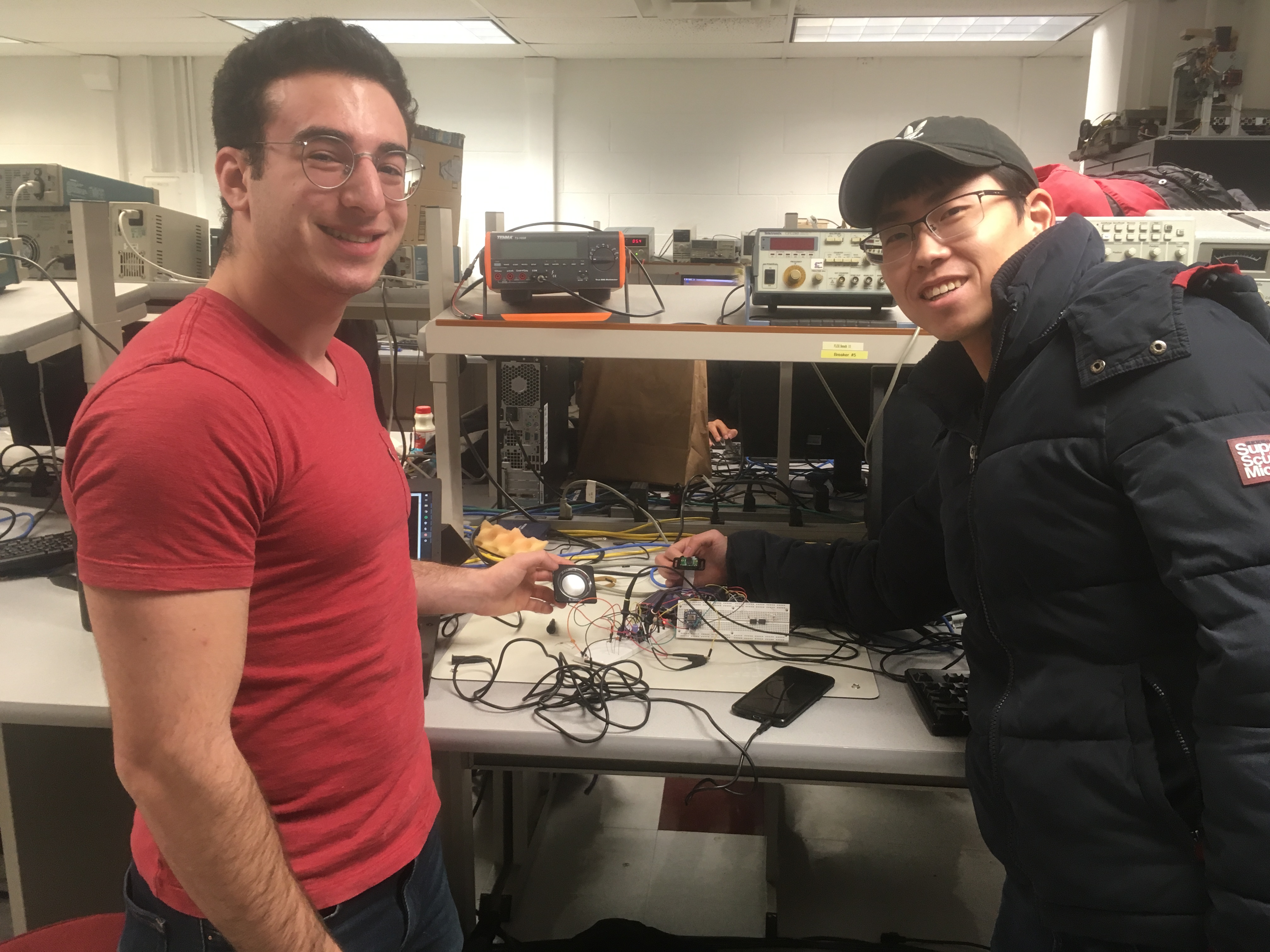
Group Photo
Project Objective
The objective of our final project is to develop an automatic gain control system, which includes a Raspberry pi model 3, an audio amplifier, an analog to digital converter (ADC), a digital to analog converter (DAC), and a speaker. Our primary goal is to build a system that can protect speakers by reducing the gain on the audio amplifier when distortion is detected, and increasing gain once it is safe to do so. The second goal is to create an automated DJ that is able to detect people and the temperature in the room so that we can determine what type of music we should play. We view this project as an embedded system that could be added onto a more powerful amplifier in order to protect expensive passive speakers.
Introduction
Audio distortion can damage speakers, and its presence, or significance, can often be reduced by decreasing the gain of the system. The automatic gain control system aims to detect distortion at the output of an amplifier, decrease the gain, and then recover the gain to the previous level when the distortion has subsided. We also expanded our project with a pi camera and thermal camera which we intended to work as an auto DJ system, but were not able to integrate this component due to limitations that will be discussed later.
Design
Audio
At the beginning of the project, we planned to use the LM386 audio amplifier to drive the speaker because it is a cheap power audio amplifier. We followed the datasheet1 and assembled the circuit shown in Figure 1. We powered the amplifier with a 9V power supply and tested a sine wave input using a function generator, but could not generate a clean output. Figures 2 and 3 show two different signal outputs the amplifier circuit generated, with the input sine wave in yellow and the output in blue. We tried to debug the circuit by changing capacitor and resistor values, and even tried using a different LM386 chip, but could not generate a clean, amplified signal. Therefore, we decided to use the TDA4052A audio amplifier chip instead of the LM386.
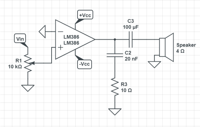
Figure 1: LM386 Audio Amplifier Circuit
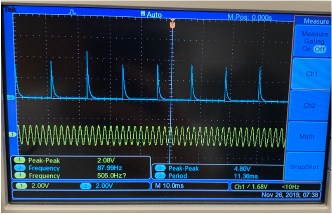
Figure 2: LM386 Output
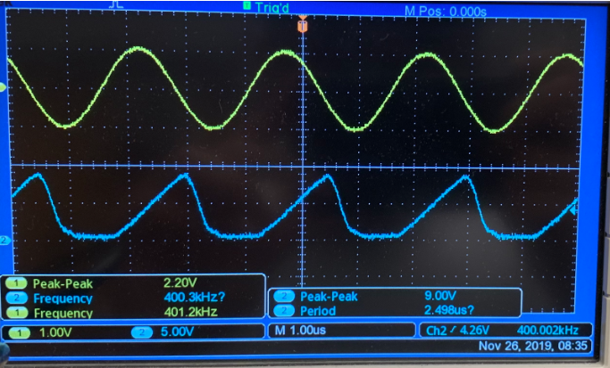
Figure 3: LM386 Output
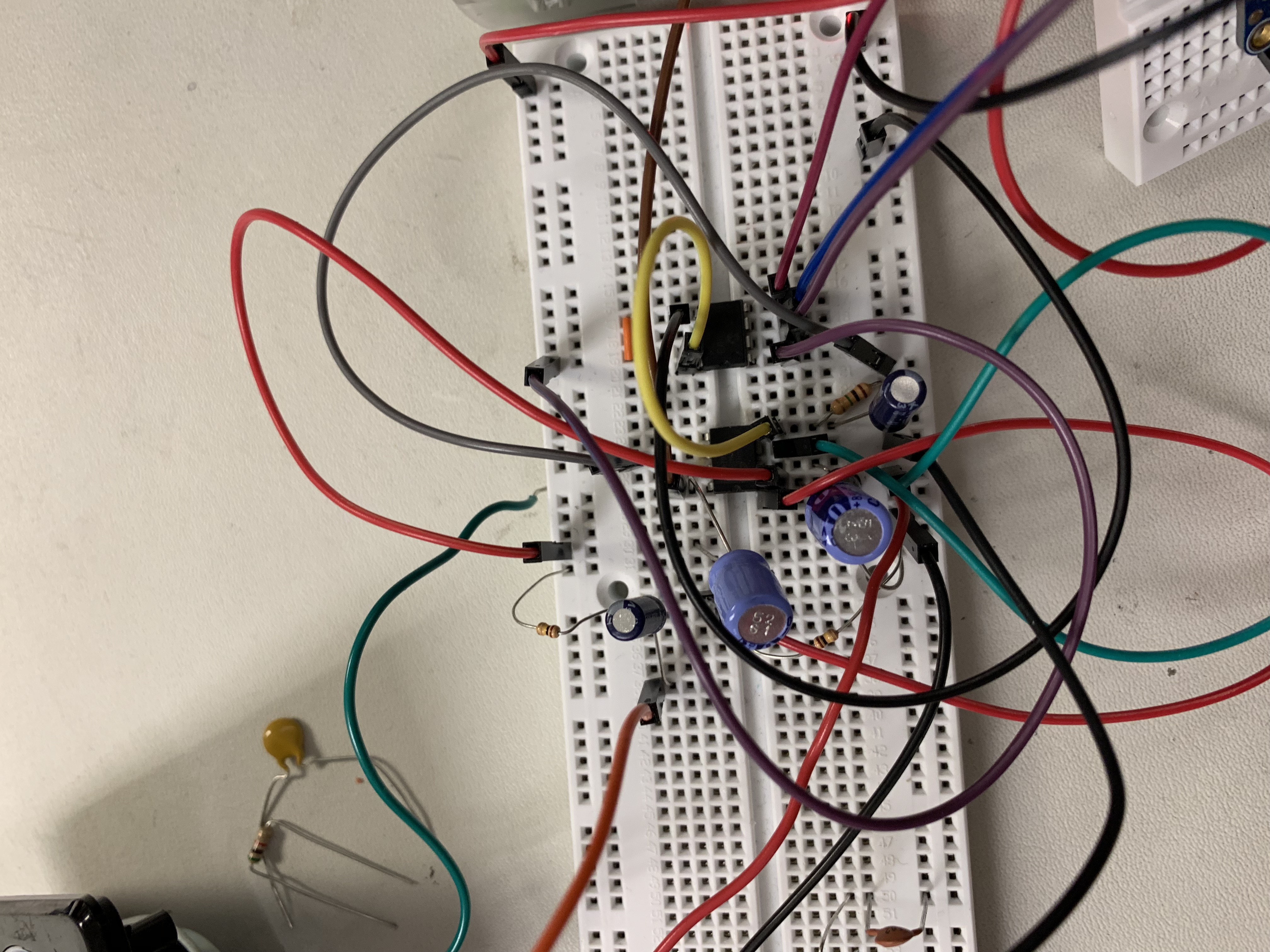
Using the TDA4052A audio amplifier with the circuit shown in Figure 4, we were able to generate a clean audio output signal with a maximum voltage gain of ~35 dB and good stability. Initially, we powered the amplifier using ±9 V, but ended up powering the amplifier directly from the Pi. This helped ensure that the amplifier would produce some visible distortion at peak input from the audio jack of the Pi, simplified powering it, and eliminated the need for a level shifter circuit on the output. The output of the audio amplifier is connected to the MCP3008 ADC chip, which is configured to take inputs from 0 to 5 V. The output is also connected to a 3W, 4Ω speaker through a 100 µF capacitor.
When we first tried to drive the signal to the ADC using amplified audio from the Pi instead of a function generator, the ADC overheated and burned out. After consultation with Bruce Land and an oscilloscope, we realized this was because the audio jack of the Pi oscillates around its ground, generating signals in the range of ±1 V, rather than being DC offset from ground as we assumed. Bruce Land speculated that this excessive negative voltage switches CMOS logic into an always-on latch, which can not be reset except by removing power from the circuit, allowing constant current to flow, and in our case destroying the device. From this point on, we were very careful about checking the voltage range with an oscilloscope before connecting any signal to the input of the ADC. We build a simple DC offset circuit, shown in Figure 5, to drive the audio amplifier within the 0 to 5 V range using a 10 µF capacitor and two 100k resistors.
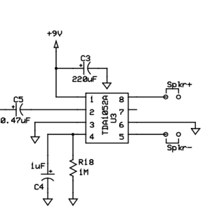
Figure 4: TDA4052A Audio Amplifier Circuit
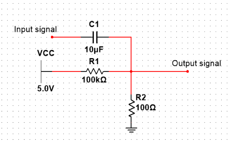
Figure 5: DC offset circuit
With the audio amplifier still powered by ±9 V, we were able to generate a clean gain of ~4x on a ground-centered input signal of 3.24 V (peak-to-peak), and started seeing some amplifier clipping after increasing the input to ~3.5 V, shown in Figures 6 and 7. When we powered the audio amplifier with 0 to 5 V instead, the maximum volume output of the Pi generated significant distortion, which allowed us to effectively test our system.
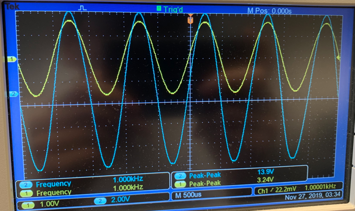
Figure 6: TDA4052A Output Signal with Sine Wave Input
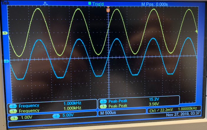
Figure 7: TDA4052A Slightly Distorted Output with Higher Amplitude Input
The final circuit is shown below.
While there can be many sources of distortion, our system is designed specifically to detect clipping, which is a common primary source of distortion. In amplifiers, clipping occurs when the output signal starts to get close to the supply and ground voltage (referred to as rails). Since the amplifier cannot output voltages outside the rails, any input that will create an output outside of the rails will actually be set to the voltage of the rail. In real amplifiers, the behavior is less idealized, and some soft clipping will occur before the voltage rails are actually reached. Figure 7 shows this phenomenon on the lower end of the signal. Even though the peak-to-peak supply of the amplifier is 18 V, the bottom peak of the sine wave starts to saturate into an almost flat region. Increasing the input voltage further would cause the output voltage to continue to increase, while saturating more, eventually converting the sine wave nearly into a square wave. Figure 8 shows the output of the TDA4052A with an input signal that is very clipped. Although the amplifier is supplied with the 5 volt line on the Pi, the peak-to-peak signal is 4.36 V. This can also be seen on the histogram generated using the ADC — the clipped peaks are offset by about 15 from the absolute maximum and minimum, even though the ADC has the same voltage supply as the amplifier.
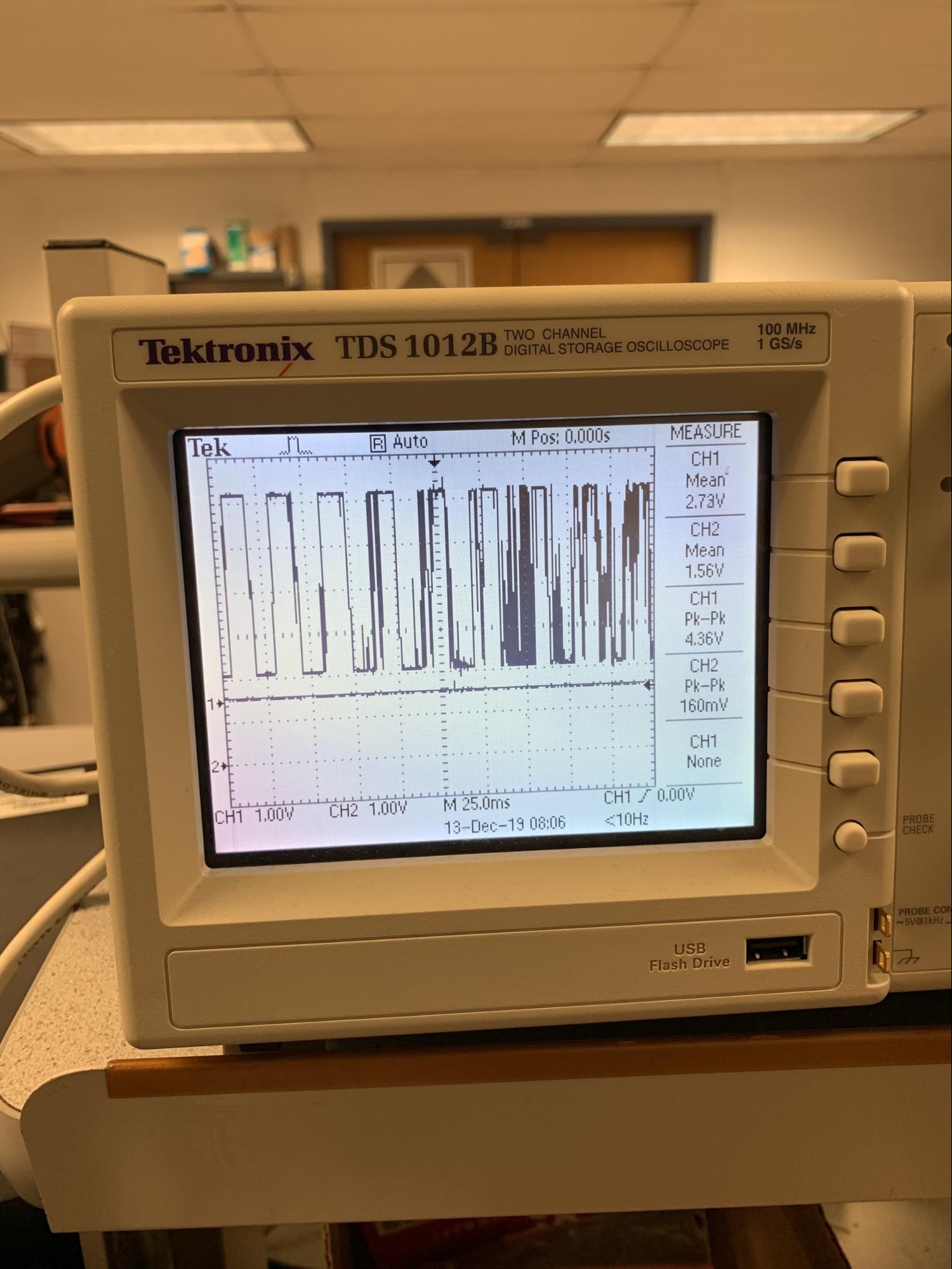
Figure 8: Clipped Audio Signal
We based our clipping detection algorithm on a paper by Christopher Laguna and Alexander Lerch, An Efficient Algorithm for Clipping Detection and Declipping Audio. They claim that by looking at a histogram of the amplitudes in an audio samples, it is possible to detect whether that signal is clipped — and consequently, distorted. A normal audio signal (Figure 9) will look similar to a Gaussian pulse, with most of the samples distributed close to the mean of the signal, and fewer samples farther away from the mean. A clipped signal, on the other hand, will have peaks near the maximum and minimum of the signal. Figure 10 and figure 11 respectively show a moderately clipped and an extremely clipped signal.
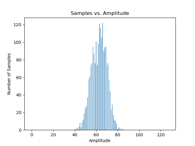
Figure 9: Non-Clipped Histogram of an Audio Sample
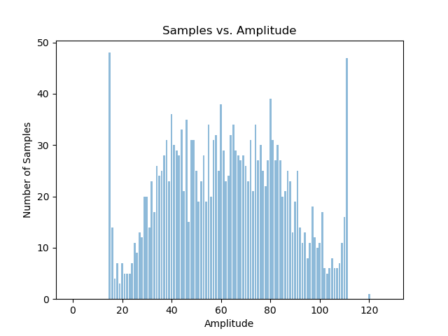
Figure 10: Moderately Clipped Histogram of an Audio Sample
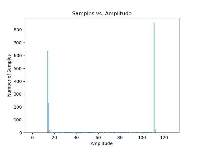
Figure 11: Very Clipped Histogram of an Audio Sample
Music is fairly complex, and can very rapidly vary between these three kinds of histograms, depending on the song. As seen in Figure xa, while the audio input is very clipped at the beginning and holds almost no meaning, the second half of the signal has much more information. Looking at the more typical audio signal in Figure 13 illustrates this idea more clearly. Even though this signal already has our gain control applied to it, it still sounds like and resembles the song it comes from. The signal has rapidly changing amplitudes, with some periods of great amplitude and some very short periods with almost zero amplitude. In the periods of zero amplitude, it would seem logical (from a computer’s limited, untrained perspective) to increase the gain as much as possible, but this will likely cause a section soon after to clip. Our algorithm seeks to avoid excessive, very rapid changes to gain, and instead hopes to maintain an audio experience as similar as possible to the original soundtrack, at original volume, if it will not cause amplifier clipping, thus sounding either bad, or completely incomprehensible, and also protecting passive speakers from being completely destroyed.
Our initial goal was to have the Pi control the whole system — being responsible for streaming the audio from Spotify, reading the ADC, running the distortion detection algorithm, and dynamically adjusting the volume output from the Pi in order to eliminate clipping. Unfortunately, we based the ADC read script on an example from the PiGPIO website (http://abyz.me.uk/rpi/pigpio/), which uses bit-banged SPI. The Pi generates audio using a PWM peripheral, and so the default for PiGPIO during normal operation is to use the PCM peripheral, but using waves or hardware PWM uses both peripherals, preventing audio from being generated. We discovered this issue too late to recover from it, and use the Pi only for the control, playing audio out from a cell phone instead. This complicates the gain control aspect, since the amplifier itself now needs to be modified. Since the PWM output is used by PiGPIO, we use the MCP4822, a 12-bit SPI DAC, to change the input to the DC volume control pin of the TDA4052A. To further complicate things, the volume control is not linear — the gain control diagram from the TDA4052A datasheet is shown in Figure 12. The x-axis shows the voltage input to the volume control pin (pin 4) and the y-axis shows the corresponding gain in decibels. Most of the control range we use falls between ~.97 volts and 1.5 volts, which we determined by listening to the sound quality at different levels. At around 1 volt, no song we listened to at full input volume sounded distorted, so we set this as the minimum threshold, as volume decreases drastically as the voltage decreases any further, and this effect is undesirable. The MCP4822 generates an output range of 0 to 2.048 volts in standard mode, and the actual voltage output is VOUT=2.048*Din/4096 V, where Din is a value between 0 and 4095.
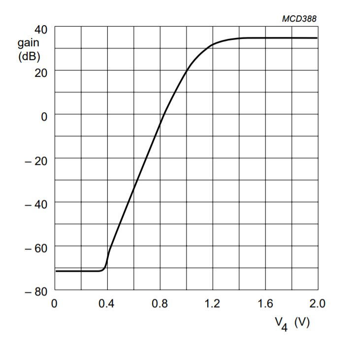
Figure 12: Gain as a Function of DC Volume Control, from the TDA4052A Datasheet
The actual code is laid out into two C programs: one to handle device I/O for the ADC and DAC, and one to process the ADC input and perform clipping detection. There are two FIFOs connecting the programs, a data and control FIFO, so that each file can send and receive data from the other. The I/O process writes the value read by the ADC to the control FIFO every time it finishes a reading. The control process reads this FIFO, then creates a histogram and runs a distortion detection algorithm, determining a gainTarget in DAC units, which it sends to the I/O process. The I/O process performs a non-blocking read of the control FIFO, and adjusts the gain written to the DAC by incrementing or decrementing by 1 if the gain has not yet reached the gainTarget. This allows the control process to compute a gainTarget infrequently, and the I/O process to make a smoother transition in gain that won’t create significant discontinuities.
The device I/O process, rawMCP3008_v2.c in our github, handles all the SPI transactions using the PiGPIO library. The base script was downloaded from the examples section of their documentation website, and was modified to only read one ADC and use different pins. Pins 5, 12, 13, and 26 were chosen, since they do not conflict with any other pins in use. SPI has a slave/chip select line, which allows multiple devices to be communicated with individually over the same clock and data lines. The Raspberry Pi 3B has one hardware SPI channel with two slave select pins. The two pins are referred to as channels, and the PiTFT uses channel 0, which is labelled as CE0 (chip enable) on the header breakout we use. Our initial attempt at using the SPI controller caused the console displayed on the TFT to redraw itself incorrectly, so we were under the impression that the PiTFT used both channels, which is part of why we used the bit-banged solution. When we added the SPI DAC, we needed another SPI channel, and realized that channel 1 is actually not used by the TFT, and we could use this directly with the PiGPIO SPI functions without any problems. The program generates a buffer of SPI transfers with a timing offset from each other, and repeats this buffer of transfers until it has collected a certain number of samples.
We were initially using a different, 8-bit SPI ADC, the ADC0832CCN, which has very specific timing constraints, and suggests that it needs a slightly non-standard SPI, which is why we were using the PiGPIO library for bitbanging SPI. We began modifying the example code for the MCP3008, and got the transfer working correctly, but were not able to correctly read data. At this point, we realized that an 8-bit ADC might not provide enough resolution to run an FFT (which was what we initially intended to use to aid distortion detection), and found out that Joe Skovira had the MCP3008 in stock. We then took it and were able to use it immediately with the example code we already had. In retrospect, we should have tried to use the standard SPI library, or the WiringPI SPI library, to communicate with it, but did not realize that the bit-banged SPI would be an issue until 48 hours before our demo time.
The control program, agc_v5.c in our github, was initially written in python, but after running some quick timing an analysis we abandoned python and switched to C for more dependable and fast performance. The ADC is sampled every 40 µs, resulting in a sampling rate of ~25k samples/sec, meaning that a file read, file write, and all the computation must be able to complete within this time frame. The program is written to execute as quickly as possible, and some accuracy tradeoffs were made for the sake of speed. It is likely that more accuracy could have been added, which would improve performance while keeping the execution time short enough. We designed the control algorithm from scratch by reasoning about the histogram method for clipping detection. After plotting a few histograms in python using data from our ADC, it seemed apparent that the sideband peaks were very close to the maximum and minimum non-zero value in the histogram, and the middle of these values generally had a peak as well. Our later plots reveal that this is not always necessarily the case, with the central peak sometimes being offset.
We decided to keep a continually updating array with HIST_SIZE bins, and experimented with 1024 (the number of possible unique ADC samples) and 256 bins. 256 bins provided plenty of resolution, so we kept the size smaller to improve performance. Making the array smaller can further improve performance and may still provide adequate resolution, as suggested by our plots which use 128 bins for better clarity. Every time an ADC value is read, the value is shifted right by two (to map from 0 to 1023 to 0 to 255), and the corresponding bin is accessed and incremented by 1. The value is also stored in a FIFO queue of length MAX_SAMPLES, currently 2048. When the queue is full, the oldest value is popped off and the corresponding bin is decremented by 1. If this bin goes to zero, and it is the current minimum or maximum, a new minimum or maximum value is found by traversing the array until another non-zero value is found. Once every INTERVAL cycles, currently 100, an update function is called, which checks for distortion and updates the gainTarget accordingly.
The update function first sums the bottom, middle, and top 5 entries of the array individually, then divides the top and bottom totals, respectively, by the middle entry, and stores the greater of the two values as lMax. The bottom, top, and middle are determined using the maximum and minimum values updated earlier. It would probably yield better results to search the array each time for three local maxima, one in each region, and sum the bins around the maxima, but would require significantly more array lookups and be slower. Given a sampling rate of around 25ksamples/sec, the 2048 long history yields a histogram detailing the information for about 82 milliseconds, which is barely perceptible. In order to extend this period slightly, and provide a varying running history rather than relying solely on the instant in which we analyze the histogram, while maintaining more accurate information about shorter samples, we create a buffer of size 20 which keeps track the previous 20 values of lMax, the ratio between the peaks. We use the maximum value in this array as our ultimate ratio, and use it as part of the condition to modify the gainTarget. A set of three conditionals follows. The first and last are conditionals in which to increase the gain, with the first responding to distortion, and the last decreasing gain in the case of no input signal. The first conditional will be entered if 1) lMax is greater than an arbitrary threshold, dnThresh, currently set to 1.0, 2) the gainTarget is not already at the minimum gain of 1950, 3) the width is greater than 2/3 of the total width, and 4) a counter, cnt, incremented each read cycle, is greater than an arbitrary factor of 20000 divided by the value of max(1, lMax). 1) determines whether or not distortion was detected. 2) saves a small amount of computation if the gain has already been killed by significant prior distortion. 3) ensures that the gain is not reduced by distortion which is not related to clipping, and that small inputs can not be destroyed. 4) is an interesting term which prevents the gain from tanking rapidly unless the distortion measured is unbelievably large, by using the distortion ratio as a scaling factor. Inside the loop, the counter cnt is zeroed to keep track of the time the gain was last changed, and the gain is dropped by 50 in DAC units unless it is below 2200 in DAC units, indicating the region of much higher sensitivity to input voltage. The solution here is odd, and was a somewhat random guess for nonlinear behavior, that does not actually do what we intended, but performs quite well. The gainTarget has the log of a different counter subtracted from it, but the value of this counter is zero, so this actually causes the gainTarget to overflow, having a value of 0xFFFF (since it is a short int type, sixteen bits). This sets to the gainTarget automatically to its minimum, but the gain recovers fairly quickly.
The middle conditional serves to recover some of the gain lost by the first conditional if it is safe to do so, using similar logic. The middle conditional will be entered if 1) lMax is below an arbitrary threshold, currently set to 0.9 (intentionally lower than the first threshold), OR the width is less than 1/4 of the histogram but greater than 5. The threshold is slightly smaller than the downward threshold so that a repeated sample that caused significant distortion will not clip the next time soon after. The importance of this can be understood by analyzing Figure 13. When a signal has little amplitude, the clipping detection does not work properly, since it sums a static five bins for three regions, and so lMax will not be useful information, which is the reason for the OR. 2) again is the counter with a scale factor, with a settable threshold to be different from the other, but currently set at 20000. This scale factor is currently calculated the same way as in the first conditional, except the scale factor is always fixed to 1 if the loop is going to be entered. Multiplying lMax by the factor would probably create an undesirably rapid increase in the gain. Inside the middle conditional, the counter cnt is reset, and the gain is increased by 10 if the gainTarget is less than 2500, and if it is greater it scales up aggressively.
The last conditional will decrease the gain slowly to the minimum value if the width is less than 3 and the middle bin in the histogram (determined from the maximum and minimum values) has more than half the possible values. Currently, when the AGC is in this mode, it will not increase the gain when a very small audio input is started (10-20% of max volume on a phone), but works well for more normal inputs, and quickly sets the gain to minimum when music is paused. This is done to minimize any passive buzzing of the speaker from noise. A more elegant solution would be to read the input to the audio amplifier using a different ADC channel, and turn the amplifier off completely when no input is detected, but we did not have time to implement this change. This addition would also allow another interesting method for detecting amplifier-induced distortion. The MCP3008 has a differential mode, where it returns the difference between two inputs, rather than their normal value, which could yield interesting results.
Figure 13 shows the output of our audio amplifier and the input to the DC volume control pin of the TDA4052A. Our end-to-end system works quite well, with minimal audible distortion, and the volume decently maintained.
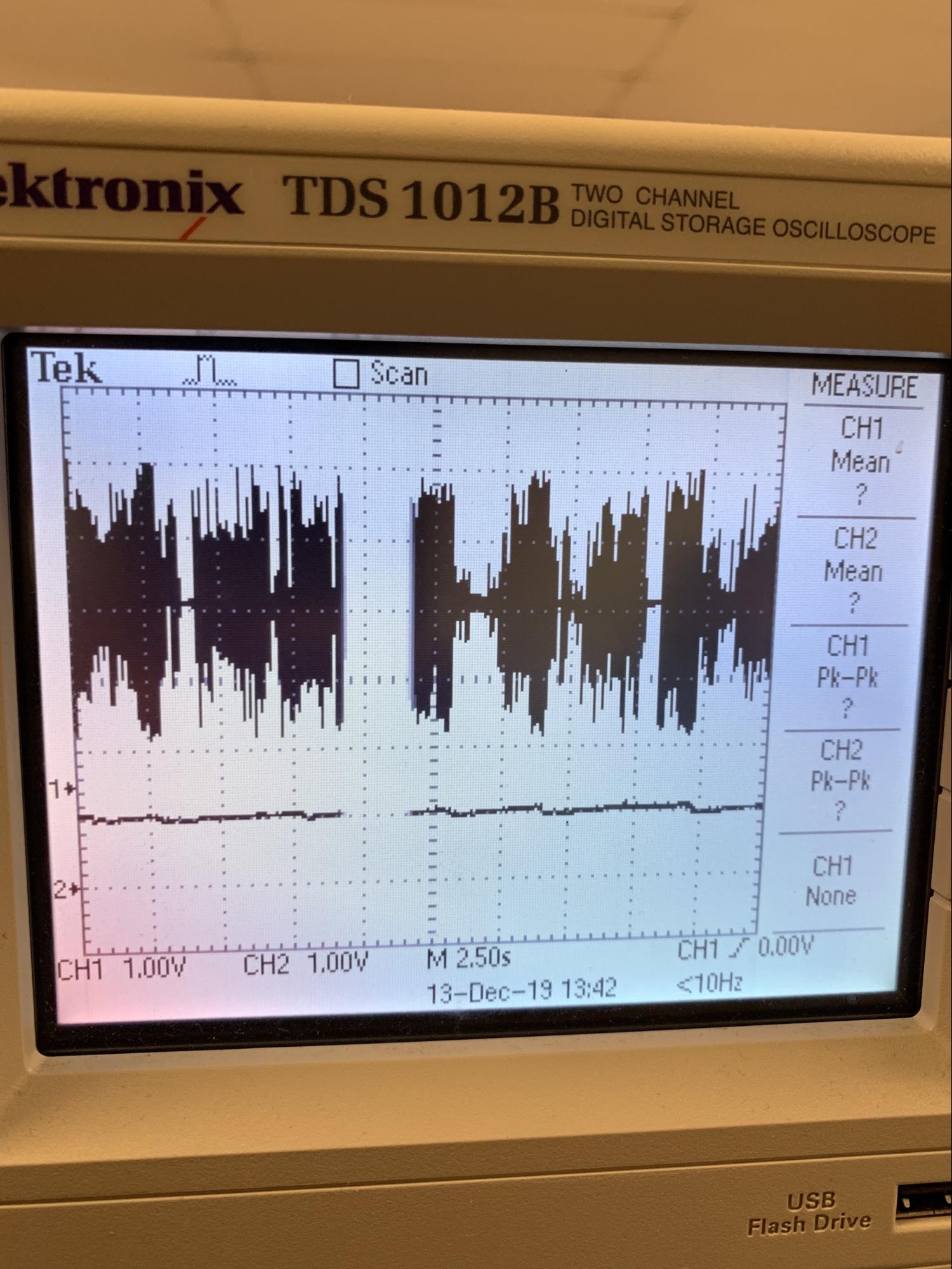
Figure 13: Oscilloscope Trace, Top Shows Audio Amp Output, Bottom Shows DC Volume Control Input
Camera:
For the auto DJ system, we planned to use OpenCV, an open-source computer vision and machine learning library. We could insert a training dataset that we would like to detect in the library and apply our own created images to the classifier for testing. Therefore, we had to install the OpenCV library on the Raspberry pi, so we followed the instructions on the PyImageSearch website5 to install it. Once the OpenCV system was installed, we found an instruction for using OpenCV face detection on the SuperDataScience website.7 We played around the code and understood how the concept worked. We then started programing and captured a single image from Picamera by using “cap=cv2.VideoCapture(0)” and the image would send into the function of face detection. The image would be converted to a gray image because the face detector expected gray images. Then, the image would test by the classifier to find a face and if there was a face, the program would draw a rectangle and insert text message on the image. Next, we worked on the program of the thermal camera. The reason that we wanted to use a thermal camera was the camera can not only monitor people but also measure the temperature of the current atmosphere. We used an Adafruit AMG8833 thermal camera which was an 8x8 array of IR thermal sensors and returned an array of 64 individual infrared temperature readings over I2C. We used CircuitPython libraries for the thermal camera and implemented the example code from the Adafruit website. Also, we assembled the circuit in the following figure for the thermal sensor.
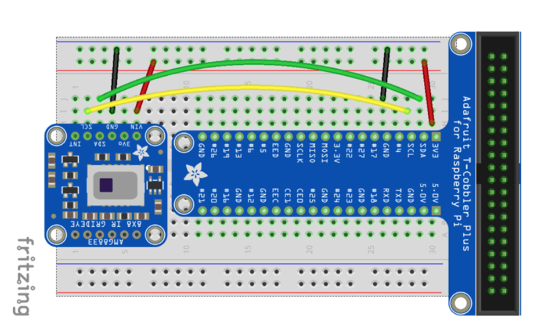
The thermal sensor connection with the Raspberry Pi.6
Once the temperature value could be successfully measured, we used pygame to visualize the temperature image. We set the maximum temperature to be color red in the array and the minimum temperature to be color purple in the array. Once each pixel has a specific color, we implemented a bicubic interpolation to make the image smoother. The example image is shown in below.

The visualization of the temperature value.
Moreover, we created an array for storing every average temperature value for each measurement and plotted the data with the corresponding index of the array to calculate the slope of the length of the music. Therefore, we could compare different slope values between each song and determine the current room atmosphere in order to adjust the music type. The program worked successfully, so we combined the face detection program with the thermal camera program together. When people’s faces were detected, the thermal camera and body detection would turn on to start to monitor the current status. The result met our expectations, but the detection performance should be optimized.
Results
Some unfortunate realizations, and a lack of early overall system testing, prevented us from achieving our project as we had initially planned, but we are still happy with the performance of the gain control itself. As discussed in the design and testing section, our initial plan was for the Raspberry Pi to be a central audio system, playing music from Spotify, detecting humans using OpenCV, and performing automatic gain control. Balancing the OpenCV workload with the other two would have required some heavy optimizations of OpenCV, which would be very interesting but probably not feasible in this time frame. The spotify aspect was abandoned because of PiGPIO taking up both the hardware PWM and PCM, preventing the Pi from playing music through the audio jack. This prevented us from combining the auto DJ system with the automatic gain control system, so we demonstrated these parts of the project separately. For the auto DJ system, the program could detect human faces and bodies at the same time. Also, the thermal camera was able to monitor the current temperature in the room and pygame could draw all the pixels into a colormap to make the data easier to process. The results are shown in the following figure. One issue was that the pictures would start to delay while the program ran for a long period because of full CPU utilization.
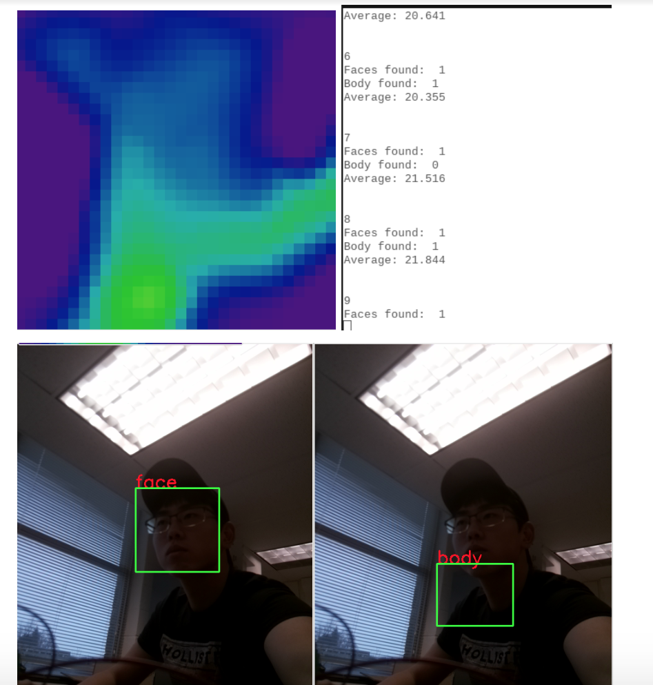
The result of the auto DJ system.
Conclusion
Our automatic gain control worked quite well, almost immediately eliminating distortion when turned on, and keeping volume output relatively steady, and close to the maximum, without allowing any perceptible distortion. There is still, of course, room for improvement. The main thing that didn’t work in this project was using PiGPIO bit-banged SPI and audio simultaneously. Another interesting thing was that two processes can not use PiGPIO at the same time, which is why we used two FIFOs instead of one. Some other strange behavior was that when opening a FIFO with the flag O_WRONLY (to write to it) without the O_NONBLOCK flag in C, that call to open would block until there was a reader of the FIFO.
OpenCV was also quite tricky to install.
Future Work
The first thing we would explore would be different options for using the ADC with SPI that would allow us to actually utilize the audio jack. If we decided the Pi wasn’t good enough, we might hook up a PIC32 and have that be responsible for the ADC and DAC (which would theoretically no longer be necessary, but could be kept).
The algorithm also has lots of room for tuning and improvements. It would be useful to get performance data and timing on all of the different components so that we could maximize the time between samples and deliver the most optimal result.
Specifically, an area we started working on but did not finish implementing was a derivative term for the gain control. In addition to the distribution of amplitudes, this could very easily tell us if a signal was flat-lined, implying that it had clipped.
Integrating Spotify would also give us plenty more inputs for the gain control algorithm, since Spotify has hundreds of different categories on which it analyzes music. These could probably be used to somehow modify parameters between different genres to maintain performance. We tested with a few different songs and genres, and the song Bass Head, a bass-heavy EDM song by Bassnectar, seemed to have the best performance, while Blues for Alice, a bebop song by Charlie Parker, an alto saxophonist. The higher frequencies of the alto saxophone sounded worse than the bass samples in Bass Head, suggesting that our tuning was more effective at detecting distortion in low frequencies than higher ones.
Group member picture
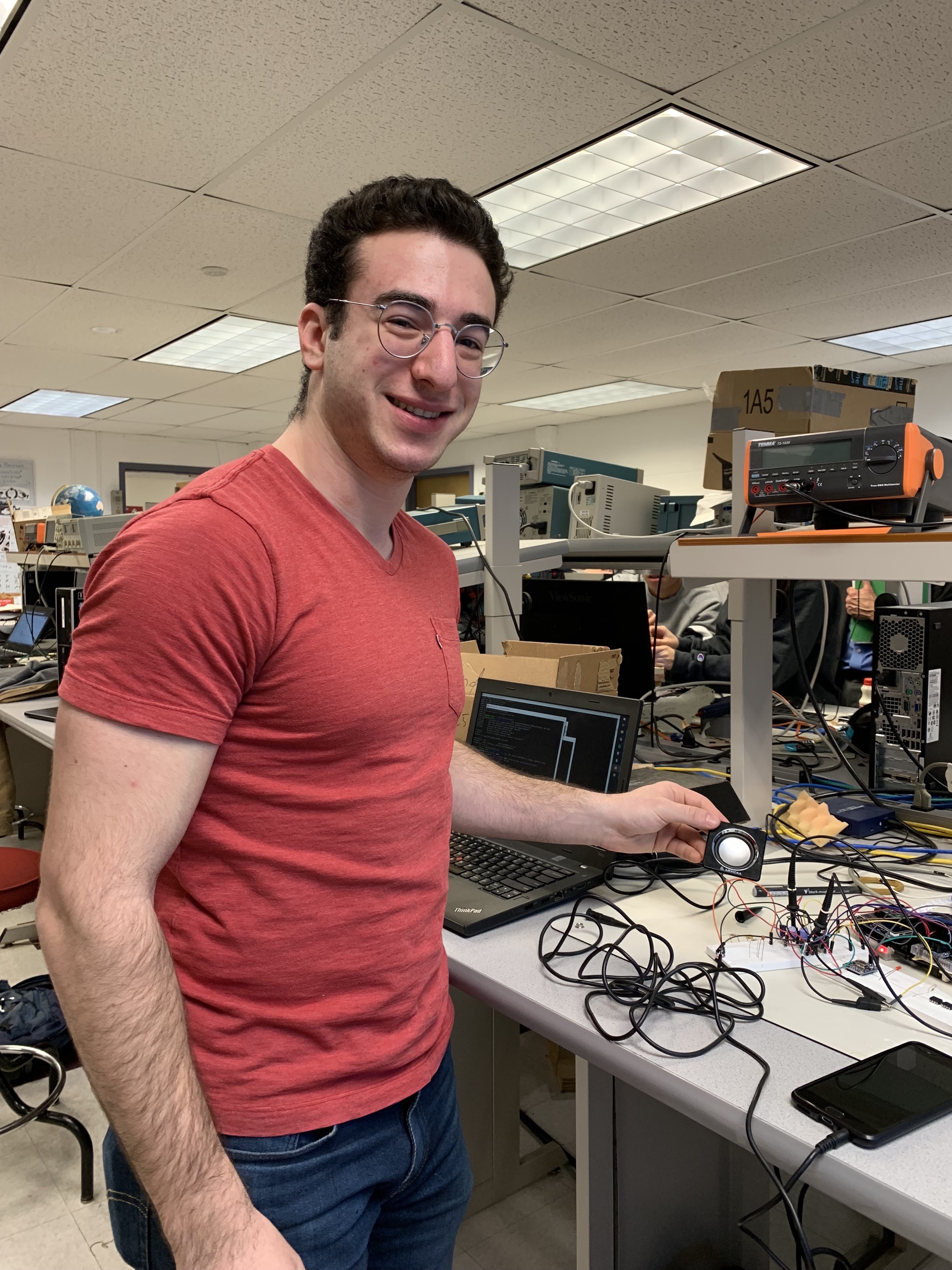
David Pirogovsky
dap263@cornell.edu
Designed the overall software architecture of the automatic gain control system.
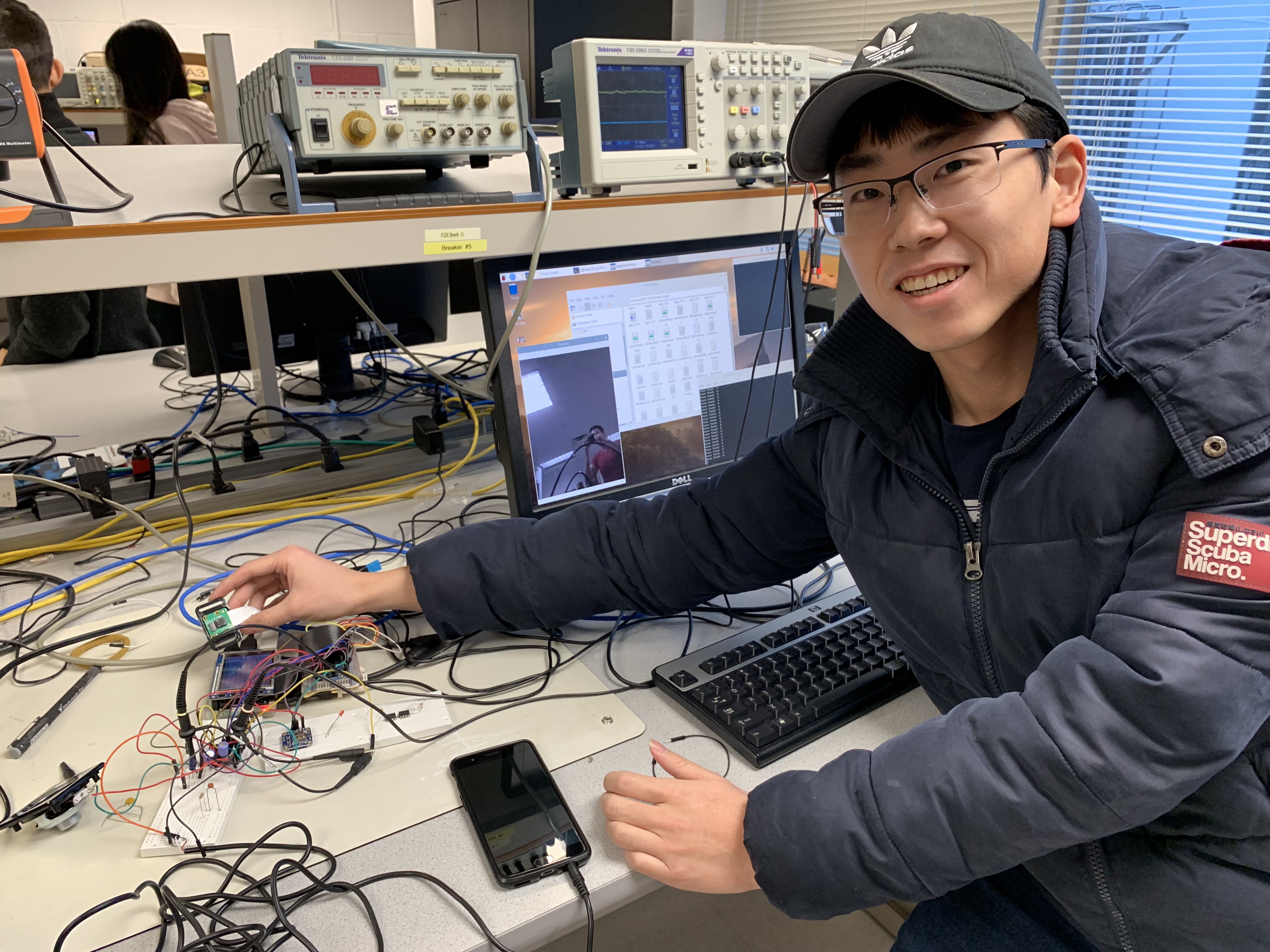
Junghsien Wei
jw2597@cornell.edu
Assembled the overall hardware circuits and designed the program of the automatic DJ system.
Parts List
- Raspberry pi $35.00
- Capacitor 100 uFx2 $3.9
- Capacitor 10 uFx2 $3.9
- Capacitor 0.47 uF $0.235
- Resistor 1M ohm $0.14
- Resistor 100 ohm x2 $0.02
- TDA4052A $0.29
- ADC0832CCN $3.06
- MCP4822 $3.00
- Pi camera $25
- Thermal camera AMG8833 $39.95
Total: $114.50
References
- Texas Instruments, “LM386 Low Voltage Audio Power Amplifier” LM386 datasheet, May. 2004 [Revised May. 2017.].
- NXP Semiconductors, “TDA7052A/AT 1 W BTL mono audio amplifier with DC volume control” TDA7052A/AT datasheet, Aug. 1991 [Revised July. 1994.].
- Rosebrock, A. (2019, November 21). pip install opencv. Retrieved from https://www.pyimagesearch.com/2018/09/19/pip-install-opencv/.
- Nuttall, B. (2018, September 27). How to work out the missing dependencies for a Python package. Retrieved from https://blog.piwheels.org/how-to-work-out-the-missing-dependencies-for-a-python-package/.
- SuperDataScience Team Saturday Jul 08, 2017. (2017, July 8). Face detection using OpenCV and Python: A beginner's guide. Retrieved December 14, 2019, from https://www.superdatascience.com/blogs/opencv-face-detection/.
- Miller, D. (n.d.). Adafruit AMG8833 8x8 Thermal Camera Sensor. Retrieved from https://learn.adafruit.com/adafruit-amg8833-8x8-thermal-camera-sensor/overview.
- Microchip, “2.7V 4-Channel/8-Channel 10-bit A/D Converters with SPI Serial Interface”, MCP 3004/3008 Datasheet [Revised Jan. 2008].
- Microchip, “8/10/12-Bit Dual Voltage Output Digital-to-Analog Converter with Internal VREF and SPI Interface”, MCP4802/4812/4822 Datasheet [Revised Jan. 2015.].
- Kerrisk, Michael. Linux man pages online. Retrieved from http://man7.org/linux/man-pages/index.html.
- National Semiconductor, "8-Bit Serial I/O A/D Converters with Multiplexer Options", ADC0831/ADC0832/ADC0834/ADC0838 Datasheet Jul. 2002. Retrieved from https://www.jameco.com/Jameco/Products/ProdDS/831200.pdf.
- Henderson, Gordon. GPIO Interface Library for the Raspberry Pi. Retrieved from http://wiringpi.com/reference/spi-library/.
- pigpio library. Retrieved from http://abyz.me.uk/rpi/pigpio/.
- DiCola, Tony. “Raspberry Pi Analog to Digital Converters.” Adafruit Learning System, https://learn.adafruit.com/raspberry-pi-analog-to-digital-converters/mcp3008.
- Lamere, Paul. Welcome to Spotipy! https://spotipy.readthedocs.io/en/latest/#.
- Laguna, Christopher and Lerch, Alexander. An Efficient Algorithm for Clipping Detection and Declipping Audio. Retrieved from https://musicinformatics.gatech.edu/wp-content_nondefault/uploads/2016/09/ Laguna_Lerch_2016_An-Efficient-Algorithm-For-Clipping-Detection-And-Declipping-Audio.pdf.
- Wilson, Adam. Pi Music Box https://www.pimusicbox.com/.
Work Distribution
David Pirogovsky
I initially assembled the LM386 circuit and did some basic testing. The output was garbage, and when I gave up I asked Junghsien to find a good audio amplifier. I then focused on setting up the ADC0832CCN, but found that Joe had the MCP3008 in his lab and moved on to using that before finishing the program for the ADC0832CCN. I then set up a FIFO for streaming values from the ADC to a python program, but decided an FFT was compute intensive and started looking into the kissFFT library. I set up an FFT successfully and took timing data for the FFT and the FIFO write, with the FFT taking ~50 milliseconds to execute and the FIFO read/write taking ~8 microseconds. Around that time, I reread Laguna and Lerch’s paper, and decided that probably be much less compute intensive and be better suited for the tight timing interval, so I began to implement that. I also spent a day or so reading through different spotify APIs and streaming methods, but did not successfully get any of them working. The rest of the time was spent working on setting up the SPI DAC, and creating, modifying, and tuning the gain control algorithm. I was satisfied with its performance in the end, and it was a pleasure working with Junghsien.
Junghsien Wei
At the beginning of the project, I helped David to assemble the audio amplifier circuit. I tested different types of amplifiers and did some simulation of non-inverting and inverting amplifiers. I figured out that using the TDA7052A audio amplifier was a good option for our project and I tested it with the function generator and oscilloscope which gave me a good performance what we want the amplifier to do in this project. Then, I focused on working the automatic DJ system by using Picamera and thermal sensor. I took several days to figure out the installation of the OpenCV and the CircuitPython. There were several errors that needed to debug. Moreover, I finished several camera programs for testing the camera performance and expanded those programs to the automatic DJ system program. David and I also spent time discussing the algorithm for the gain adjustment in the automatic gain control system. In the end, our demonstration worked well and I enjoyed working with David in this course.
All our code can be found on this github repo!